
Why build quantum computers if you can simulate them?
The advantages and limitations of modeling quantum computers

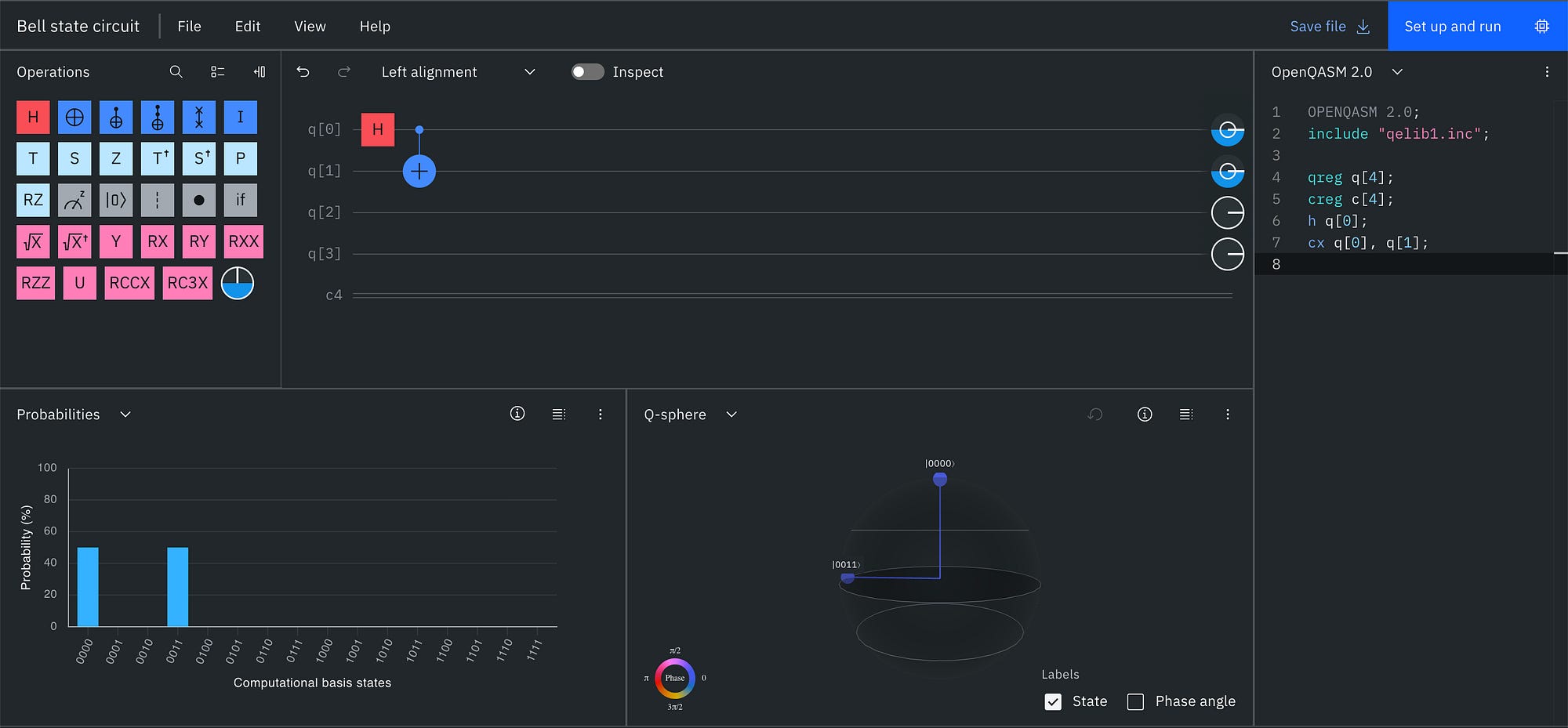
Researchers often run algorithms designed for quantum computers on classical computers that can simulate their behavior before executing them on actual quantum hardware.
Using quantum circuit simulators, such as the IBM Quantum Platform Composer, enables prediction and validation of potential results while reducing the computational time and cost often associated with running algorithms on quantum hardware.
Then, this raises the question: Why build quantum computers if you can simulate them?
High-performance classical computers are valuable for simulating smaller quantum circuits or programs. However, in practical use cases that are too complex and resource-intensive for classical computers to handle, quantum computers remain necessary.
This article explores the current thresholds and limitations of quantum computers and quantum circuit simulators and when it is appropriate to use either.
What is a quantum circuit simulator?
A quantum circuit simulator is a software platform accessed on a classical computer (i.e., a laptop) that allows you to run quantum circuits, or software programs that can run on a quantum computer, as if they were running on a quantum computer.
Popular web-based quantum circuit simulators include IBM Quantum Circuit Composer, Cirq, and BlueQubit Simulator. Popular libraries include the cuStateVec library in the NVIDIA cuQuantum SDK and the PennyLane SDK.
Quantum simulator vs. quantum circuit simulator
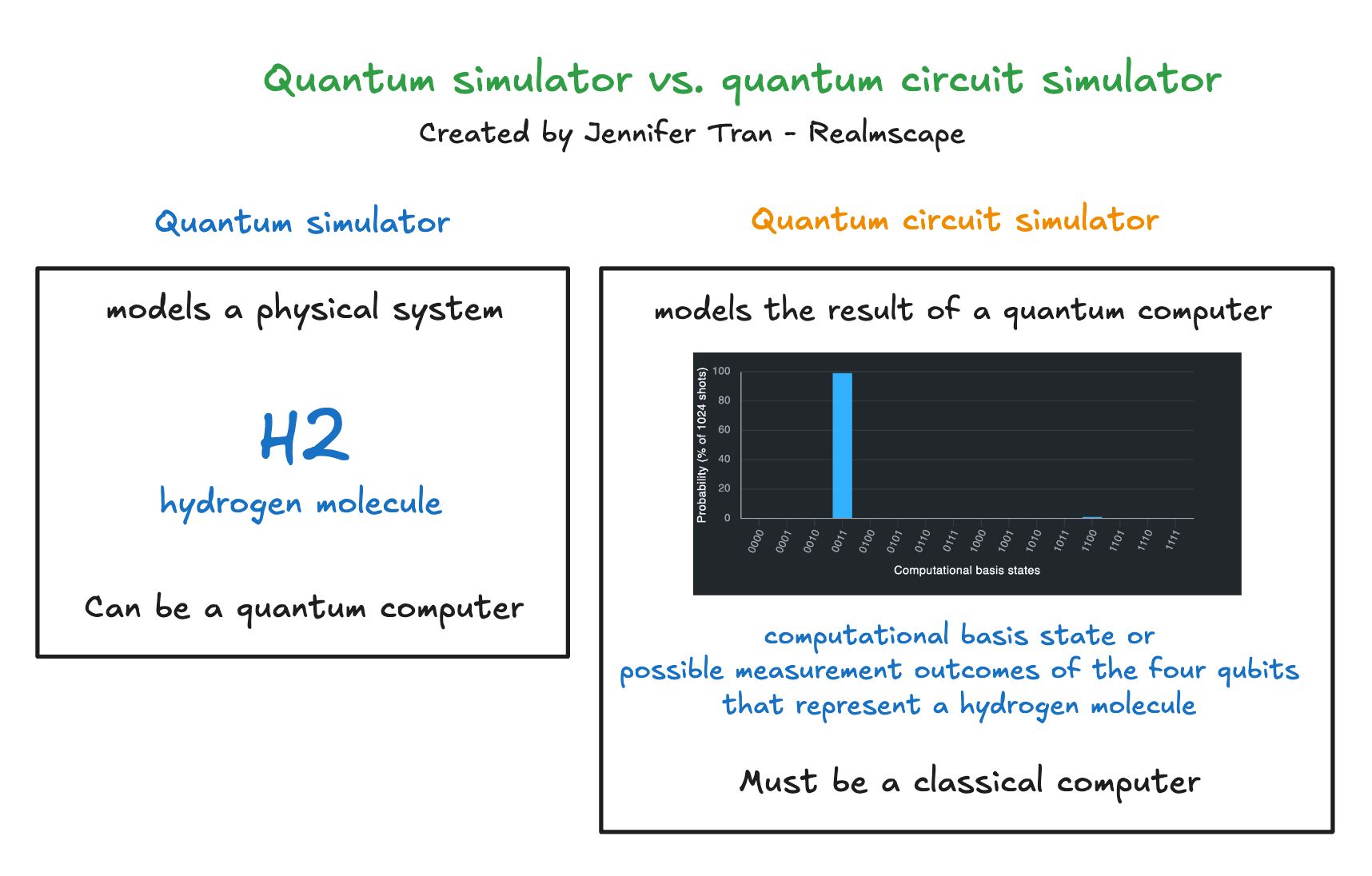
A common misconception is that quantum circuit simulators are quantum simulators, but they are fundamentally different.
A quantum simulator is a broad term for a tool that models complex physical systems. For example, a quantum simulator is used to model the atoms of a chemical molecule that scientists use to research new materials. Quantum computers are often used as quantum simulators.
In contrast, a quantum circuit simulator models the behavior of a quantum computer, including its state, on a classical computer using well-defined mathematical logic. For example, a quantum circuit simulator can model a result similar to that a quantum computer would produce when acting as a quantum simulator of a chemical molecule.
A quantum simulator can be a quantum computer, but a quantum circuit simulator cannot.
Limitations of quantum circuit simulation
Quantum circuit simulators face limitations as circuit sizes (in qubits and gates) grow, because they require excessive data storage and the mathematical calculations they perform to model quantum computers become too complex.
At present, quantum circuit simulators can handle only a maximum of 30–50 qubits and are unable to fully replicate even today’s cloud-accessible quantum computers of 100–200 qubits. To run a useful practical algorithm, at least 100 qubits are necessary [4].

Major memory requirements
First, classical computers are limited by random access memory (RAM) available to store all possible quantum states.
A state vector circuit simulator, the most common implementation of a quantum circuit simulator, stores the quantum state of each qubit as a state vector.
The state vector space grows exponentially with the number of qubits, making it too large for classical computers to handle. If you are interested in a deeper dive into quantum states, please refer to this article.
Each state vector contains two complex numbers representing the probabilities that the qubit is in states 0 and 1. Therefore, a system requires two complex numbers per additional qubit.
Each complex number requires 16 bytes of RAM. Since each qubit requires a state vector of two complex numbers, the state vector for each qubit requires 32 bytes of RAM. A simple formula to calculate the required RAM to simulate a system is 2^(N+4) bytes, where N is the number of qubits [1].
The RAM requirements for a state vector circuit simulator are manageable with fewer qubits, but are impractical as the number of qubits scales.
Two qubits require 64 bytes, which is the equivalent of a 64-character text message.
# RAM in bytes for two qubits

2^(N+4) with N as the number of bytes
2^(2+4)
2^(6)
64 bytes
Thirty qubits require 17,179,869,184 bytes, or 17 gigabytes of RAM, which is the equivalent of the lowest-tier MacBook Pro.
2^(30+4) = 2^34 = 17,179,869,184 bytes or 17 gigabyesOne hundred qubits require 2.028241 x 10³¹ bytes or 2.02824096 × 10²² gigabytes, which is more than all of the RAM space available in the world. A state vector circuit simulator could not replicate even the largest quantum processor currently available to users.
2^(100+4) = 2^104 = 2.028241 x 10^31 bytes or 2.02824096 × 10^22 gigabytesThe development of quantum computers remains necessary because classical computers cannot simulate them at scale, particularly for future use cases requiring hundreds or thousands of qubits.
Complicated mathematics
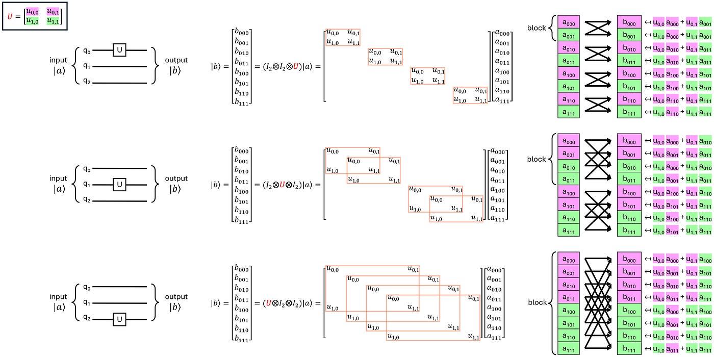
The complexity of the mathematical calculations also grows exponentially with the number of qubits and gates (logic operations applied to qubits).
In state vector simulators, qubits and gates are represented as matrices, requiring complex multiplication as more are added.
As an example, here is a matrix of two qubits, where the first qubit is in the initial state of |1> and the second is in the ground state |0>:
              ⎡ 0·1 ⎤   ⎡ 0 ⎤
              ⎢ 0·0 ⎥   ⎢ 0 ⎥
|1⟩ ⊗ |0⟩  =  ⎢ 1·1 ⎥ = ⎢ 1 ⎥ = |10⟩
              ⎣ 1·0 ⎦   ⎣ 0 ⎦
Here is the matrix of a controlled NOT (CNOT gate), which changes the state of the target (second) qubit to the opposite of the control qubit’s state only if the control qubit’s state is |1⟩.
       ⎡ 1  0  0  0 ⎤
CNOT = ⎢ 0  1  0  0 ⎥
       ⎢ 0  0  0  1 ⎥
       ⎣ 0  0  1  0 ⎦
To apply a CNOT gate to the two qubits, the following matrix multiplication is applied.
       ⎡ 1  0  0  0 ⎤ ⎡ 0 ⎤   ⎡ 0 ⎤
CNOT = ⎢ 0  1  0  0 ⎥ ⎢ 0 ⎥ = ⎢ 0 ⎥ = |11⟩
       ⎢ 0  0  0  1 ⎥ ⎢ 1 ⎥   ⎢ 0 ⎥
       ⎣ 0  0  1  0 ⎦ ⎣ 0 ⎦   ⎣ 1 ⎦
As the number of qubits and gates grows, classical computers struggle to keep up with the matrix multiplication involved. This cost grows exponentially, described by O(m·2^(2N)), where N is the number of qubits and m is the number of gates [1].
Types of quantum circuit simulation in practice
Various types of quantum simulation tools exist but the same code is used to model a physical system on a quantum simulator and to show the state of a quantum computer using a quantum circuit simulator.
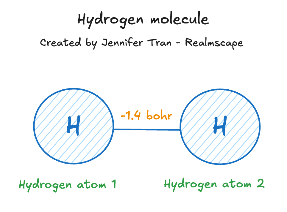
The following Python code snippets, using the PennyLane SDK to model two hydrogen atoms separated by 1.4 Bohr, representing the most stable bond to form a hydrogen molecule, require four qubits and can either run on a quantum computer or a quantum circuit simulator.
import pennylane as qml
from pennylane import numpy as np

# Describes two hydrogen atoms that are -1.4 Bohr apart

symbols = [”H”, “H”]
coords  = np.array([[0.0, 0.0, 0.0],
                    [0.0, 0.0, 1.4]])

# Translates the hydrogen molecule into something a quantum computer understands
# H represents the total energy system of the molecule
# n represents how many qubits the molecule needs

H, n = qml.qchem.molecular_hamiltonian(symbols, coords, basis=”sto-3g”, method=”dhf”)
This code runs the Variational Quantum Eigensolver, a popular algorithm for finding the ground state of physical systems, in this case, the ground state of a hydrogen molecule.
def prepare(theta):
    qml.BasisState(start, wires=range(n))
    qml.DoubleExcitation(theta, wires=[0, 1, 2, 3])

# measures the energy of the molecule
@qml.qnode(qc)
def energy(theta):
    prepare(theta)
    return qml.expval(H)

# measures the state of the molecule
@qml.qnode(qc)
def state(theta):
    prepare(theta)
    return qml.probs(wires=range(n))

# Uses the Variational Quantum Eigensolver (VQE) to turn
# the different parameters until the energy is as low as it goes
theta = np.array(0.0, requires_grad=True)
opt = qml.GradientDescentOptimizer(stepsize=0.4)
for _ in range(40):
    theta = opt.step(energy, theta)

# The ground state that a quantum simulator or quantum circuit simulator finds
E_found = float(energy(theta))
E_exact = float(np.linalg.eigvalsh(qml.matrix(H, wire_order=range(n)))[0])
The main difference in the code is that these lines specify which type of “simulator” we would use, choosing either an actual quantum computer or a quantum circuit simulator running on a classical computer.
# Defines the simulator that we would use (choose one or the other)

# 1. uses a IonQ Forte1 quantum computer that is accessible through Amazon Web Services (AWS)
device_arn = “arn:aws:braket:us-east-1::device/qpu/ionq/Forte-1”
qc = qml.device(”braket.aws.qubit”, device_arn=device_arn, wires=n, shots=1000)

# OR 2. uses the default built-in quantum circuit simulator that uses a classical computer
qc = qml.device(”default.qubit”, wires=n)
Running the full code on different types of simulators follows a similar process but can yield different results and requires different resources.
Running this example on an IonQ Forte1 quantum computer via Amazon Web Services (AWS) Braket would require more than $74.
The current on-demand rate is $0.30 per task + $0.08 per shot per task (the number of times a task is run). With six separate tasks in the full script and an optimal of 150 shots for a smaller VQE circuit, the estimated cost is nearly $74 [2].
Rate for on-demand access to IonQ Forte1 device: $0.30 / task + $0.08 / shot per tasks

Number of tasks: 6
Number of (optimal shots); 150
($0.30 * 6) + ($0.08 * 6 * 150)
$1.80 + $72.00 = $73.80
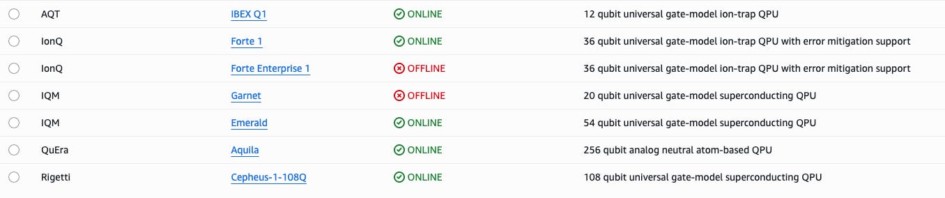
A dedicated quantum computer could execute the program in seconds to minutes, but dedicated reserved time of an IonQ Forte1 would cost $7,000 per hour on AWS. Most developers would opt for shared cloud quantum resources, which means quantum circuit execution can take hours due to queuing hundreds or thousands of requests, as shown on the IBM Quantum Platform status tracker.

Since I did not want to pay $74, I “cheated” and used DM1, an AWS simulator that includes noise, or disturbances commonly encountered in quantum computers. A simulator that integrates noise simulates a quantum computer more closely than ones that do not, such as a universal state vector simulator, the most common implementation of a quantum circuit simulator.
Using the DM1 simulator saved a considerable amount of time and money compared to a real quantum computer; it cost $0.0225 and took 18 seconds to run.
# uses DM1 AWS quantum simulator as device to run the circuit
device_arn = “arn:aws:braket:::device/quantum-simulator/amazon/dm1”
Modeling H2 uses 4 qubits.
GROUND-STATE ENERGY
ideal (no noise) : -1.13728 Hartree
DM1 (with noise) : -1.08274 Hartree
THE MOLECULE’S QUANTUM STATE (noisy)
0011 probability 0.80%
0100 probability 1.70%
1000 probability 1.40%
1100 probability 92.30%
1101 probability 1.90%
1110 probability 1.50%
1111 probability 0.20%In general, since the circuit requires only four qubits, all quantum circuit simulators should produce a similar result.
Next, I ran the result using the default built-in state vector quantum circuit simulator in the PennyLane SDK, which is free and provides instant results.
A state vector simulator returns the same result each time because it applies deterministic mathematical operations to the state vector based on the gates in the circuit. The next section explains how using predetermined mathematical logic in quantum circuit simulation limits its capabilities.
Compared to the DM1 result, the result using the default state vector quantum circuit simulator in the PennyLane SDK was more precise, with fewer chances of varying quantum states, due to the lack of noise:
Modeling H2 uses 4 qubits.

GROUND-STATE ENERGY
  quantum circuit simulator found: -1.13728 Hartree
  known exact answer: -1.13728 Hartree

THE MOLECULE’S QUANTUM STATE
  (each row is one way the 2 electrons can sit in the 4 orbital-slots)
    0011   probability  1.27%
1100 probability 98.73%Researchers working with circuits that have fewer qubits, such as this example, benefit from more accessible, faster, and cheaper simulations rather than running circuits directly on quantum hardware. However, as their circuits grow, they will encounter limitations with quantum circuit simulators.
Conclusion
High-performance classical computers are valuable and effective for simulating smaller quantum circuits or programs, like the four-qubit example in the article. Using the built-in state vector simulator returned an exact ground-state energy instantly and for free, while running the same circuit on an IonQ Forte1 would have cost nearly $74.
However, classical simulation becomes too mathematically complex and resource-intensive as the number of qubits in consumer-accessible quantum computers grows. At 30 qubits, a simulator already requires 17 gigabytes of RAM; at 100 qubits, it would require more RAM than exists in the world.
So, why build quantum computers if you can simulate them? For practical use cases that will require hundreds or thousands of qubits, classical simulation is too complex and resource-intensive, and quantum computers remain necessary.
Additional Resources
Xu, X., Lee, J. S., & Lim, Y. S. (2023). A Herculean task: Classical simulation of quantum computers (arXiv:2302.08880). arXiv. https://arxiv.org/abs/2302.08880
Bisicchia, G., Bocci, A., Pimentel, E., & Brogi, A. (2026). How many shots are enough for a quantum circuit? (arXiv:2606.16965). arXiv. https://arxiv.org/abs/2606.16965
McGuffin, M. J., Robert, J.-M., & Ikeda, K. (2025). How to write a simulator for quantum circuits from scratch: A tutorial (arXiv:2506.08142). arXiv. https://arxiv.org/abs/2506.08142
Preskill, J. (2018). Quantum computing in the NISQ era and beyond (arXiv:1801.00862). arXiv. https://arxiv.org/abs/1801.00862