
How to create a quantum circuit
A beginner’s guide to quantum circuits, the equivalent of digital circuits in quantum computing

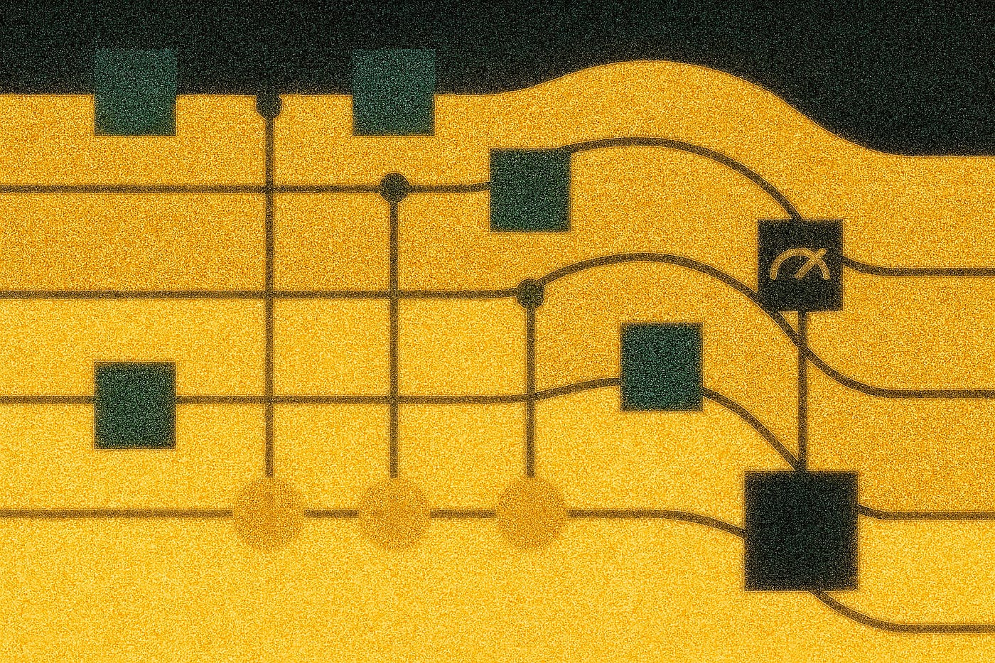
During this year’s IBM Qiskit Fall Fest, I saw a diagram of a quantum circuit that was similar but less abstract than the one above, and I have been figuring out its components ever since.
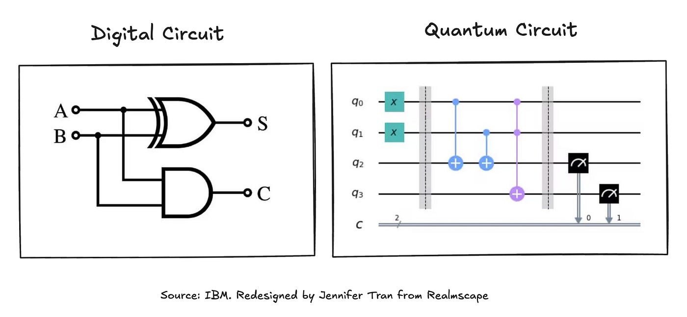
A quantum circuit is the quantum computing equivalent of a digital circuit, which is the foundation of all computers. Similar to a digital circuit diagram, a quantum circuit diagram is a visual representation of the logic and operations underlying an algorithm that can run on a quantum computer.
This article compares and contrasts quantum circuits with digital circuits and explains how to create a quantum circuit diagram using simple, practical quantum computing examples.
Digital circuits vs. quantum circuits
A quantum circuit is the quantum computing counterpart to a digital circuit in everyday classical computing. They are similar because they are each other’s equivalents. However, because classical and quantum computing are fundamentally different, they are pretty distinct.
Here’s a diagram comparing a digital and a quantum circuit, showing both graphical similarities and distinct components.
Digital circuits
A digital circuit forms the basic foundation of a classical computer.
A typical computer has millions, or even billions, of digital circuits, each performing simple logical operations that add up to complex calculations and tasks. Multi-layered circuits, featuring thousands of individual circuits per layer, are standard in devices that require high reliability and complexity, such as medical instruments and high-performance computers.
An individual digital circuit processes simple rules based on smaller components known as logic gates, which perform logic operations (AND, OR, NOT).
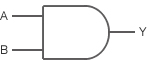
This simple OR logic gate shows that two inputs (A and B) will produce a combined output (Y). Using binary, Y is 0 when A and/or B are 0. Y can only be 1 when both A and B are 1.
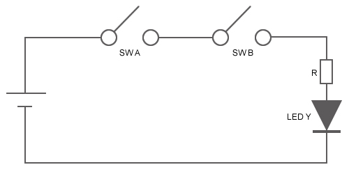
More practically, the example below demonstrates how a digital circuit with an AND gate controls the lighting of LED Y based on the binary example above. LED Y turns off (or 0) when output Y is SW A and/or SW B are off (or 0). LED Y lights up (or 1) when both SW A and SW B are on (or 1).
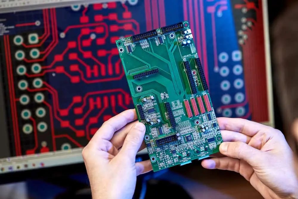
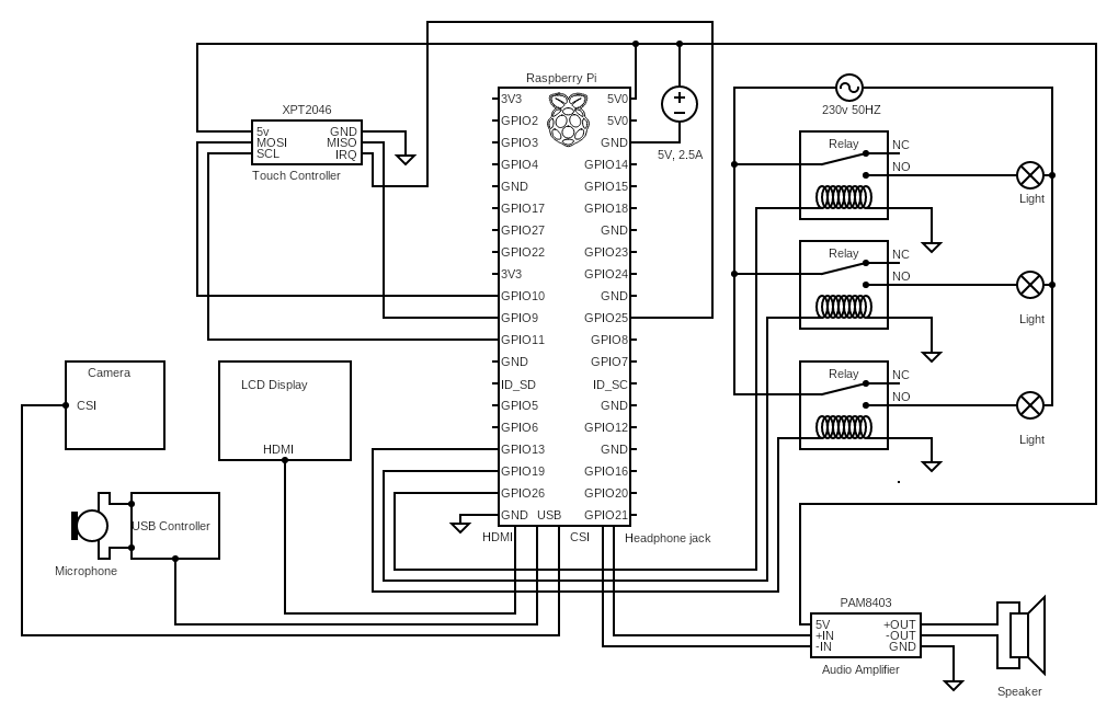
An individual circuit can perform basic operations, such as a simple light switch, but complex, meaningful tasks require many such circuits, as computers are designed to handle. The provided circuit diagram of a Raspberry Pi, a small, affordable single-board computer with a touchscreen, shows how much more complex it is compared to our light switch example.
Quantum circuits
Just as digital circuits form the foundation of classical computers, quantum circuits serve as the basis of quantum computers.
Volume of quantum circuits
Fewer quantum circuits are needed to accomplish complex quantum computing tasks, as quantum circuits have more computational power than digital circuits.
Dozens or thousands of quantum circuits compose a quantum computer, far fewer than the millions required to run an everyday computer. 100 qubits, the basic unit of information in quantum computing, is the benchmark for running an algorithm in small-scale scientific research experiments, according to IBM and Google. The largest quantum computer has 6,100 qubits. Researchers at the University of Tokyo, the University of Chicago, and IBM have committed to developing a 100,000-qubit system by 2033, which would enable practical uses, such as medical modeling and agricultural discoveries, that we currently cannot solve.
Technical Architecture
Like digital circuits, where the combined logic of individual circuits adds up to complex operations, quantum circuits define the computations that quantum computers perform.
Quantum computers consist of quantum processing units (QPUs), which are made up of quantum circuits. Quantum circuits are made of a register of qubits, and each qubit is operated on by gates that perform logic.
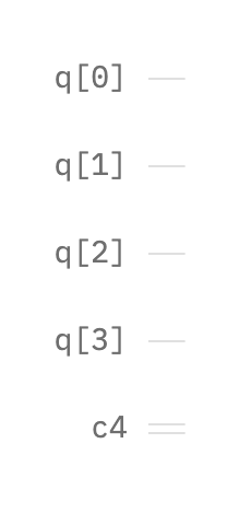
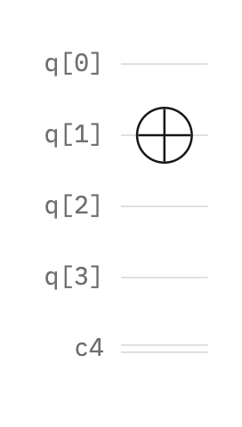
Quantum circuits also use classical components. When a state change happens, the measurement is stored in classical bits within the quantum circuit. This is shown by a “c4” line on a quantum circuit diagram.
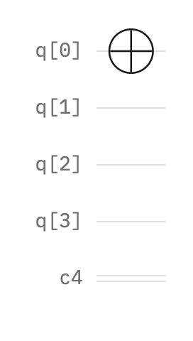
Here is an initialized quantum circuit with a register of four qubits (q[0], q[1], q[2], q[3], q[4]) and a classical register (c4).
Like in digital circuits, quantum gates perform logical operations and alter the state of the circuit. However, gates in quantum circuits are different from those in digital circuits because, unlike classical bits, qubits can be in states 0 and 1 simultaneously, and quantum computation must be reversible, or the input must be reconstructible.
Quantum computation must be reversible due to the principles of quantum mechanics. A quantum state, which includes all possible measurement outcomes of the entire quantum system, always has a total probability of 1, and this must remain true as the system evolves. To ensure that all measurement outcomes sum to 1, quantum gates must transform states in a way that preserves all information. If information were lost during computation, some outcomes might repeat, causing the total probability over all quantum states to fail to form a proper probability distribution, and the total probability would no longer equal 1 [2].
Therefore, quantum gates cannot be the same as classical gates because classical inputs can be identified or reconstructed based on their output. A good example is the previously explained light switch scenario. When the light switch is off, it is unclear whether it is off because SW A and SW B are both off, or because only one of them is off.
The number of quantum gates exceeds the eight classical logic circuits, so it is more valuable to explain some of them in applied circuit examples than to explain them individually.
Quantum circuit examples
We will explain circuit components by examining beginner quantum circuit examples using the IBM Quantum Platform Circuit Composer as a diagram tool. Many other tools for creating quantum circuit diagrams exist, including Quirk, QuantumJS, and those from the University of Stuttgart.
Simplest example
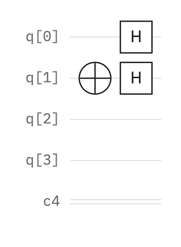
The simplest example of a quantum circuit consists of a single gate that changes the state. The example below demonstrates initializing a qubit and preparing it to start.
Qubits can be in state |0⟩ or |1⟩. Initially, qubits are in the ground state |0⟩. To initiate a qubit, it must move from this ground state to the state |1⟩. One approach is to apply a NOT gate, which inverts (switches the state to the opposite) state. This quantum circuit (q[0]) has a single NOT gate (represented by a circular target) that operates on a single qubit.
Slightly simple example
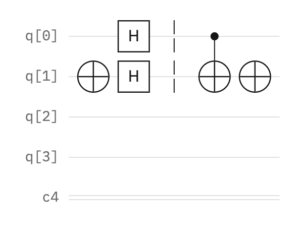
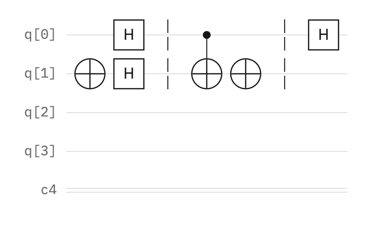
Another, more complex but still simple example is a circuit that illustrates quantum entanglement between two qubits. Quantum entanglement is when qubits become connected and correlated with each other, even when they eventually become separated by a far distance. Quantum entanglement is the phenomenon that enables operations to process multiple qubits simultaneously, making quantum computing as fast and powerful as it is.
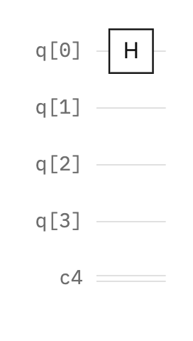
As mentioned earlier, a qubit starts at the ground state |0⟩. A qubit can simultaneously be at, or in a superposition of, states |0⟩ and |1⟩ by applying a Hadamard gate, represented as a box with the letter H.
For example, this shows qubit (q[0]) at a superposition of states |0⟩ and |1⟩:
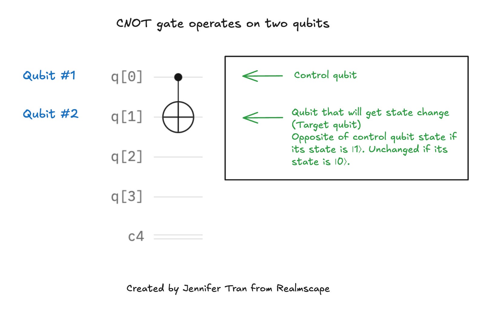
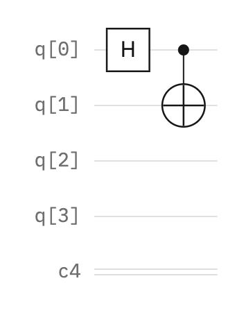
To connect or entangle with another qubit, the circuit needs to apply a two-qubit component that operates on two qubits at a time. A controlled NOT or CNOT gate takes two qubits: the first, a control qubit, and then a target qubit, and it changes the state of the target (second) qubit to the opposite of the control qubit’s state only if the control qubit’s state is |1⟩.
This final circuit example demonstrates two qubits that are entangled or have “connected” states. The first qubit (q[0]) exists in a superposition, having both |0⟩ and |1⟩ states due to the Hadamard gate. The second qubit (q[1]) is expected to be in the opposite state of the first, with a CNOT gate where the first is the target and the second is the control. However, because a superposition does not have an “opposite” state, the final state of the second qubit depends on the result of the state of the first qubit.
Algorithmic example
Like classical computing, quantum circuits require more resources for complex algorithms, involving multiple qubits and gates.
The Deutsch algorithm is one of the first quantum algorithms to prove that quantum computers are more powerful than classical computers.
An unknown function f(x) accepts only inputs of 0 or 1. It has two possibilities: constant (always returning 0 or 1) or balanced (alternating between 0 and 1). If inputting zeros and ones results in identical outputs (always 0 or always 1), the function is deemed constant. If the outputs differ (one is 0, and the other is 1), the function is considered balanced. In other words:
If you get these results when inputting 0 or 1, then the function is constant:
f(0)=0 and f(1)=0 Then f(x) is constant (always 0)
f(0)=1 and f(1)=1 Then f(x) is constant (always 1)
If you get these results when inputting 0 or 1, then the function is balanced:
f(0)=0 and f(1)=1 Then f(x) is balanced (always 0 or 1)
f(0)=1 and f(1)=0 Then f(x) is constant (always 0 or 1)
In the classical world, you would need to call the function twice: once with input 0 and once with input 1. Deutsch found a more efficient method using quantum computing. They tested the function by passing in both 0 and 1 to two qubits simultaneously, calling the function only once.
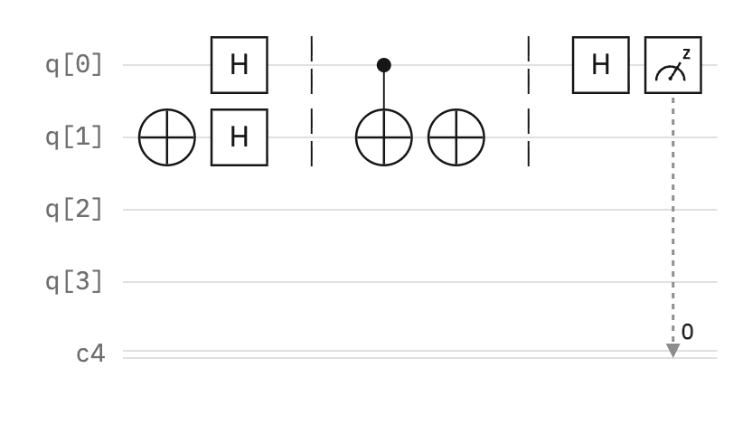
The example below demonstrates the Deutsch algorithm. It is separated into five essential steps, as explained in plain English below. Here is a helpful video if you’re looking to understand the math behind the algorithm, or a tutorial if you want to review the Qiskit code.

Step one — Initialization
To start, we need two separate qubits: one to test the function and one to handle the final measurement of the output (balanced or constant).
The first step is to start with two qubits: the one that tests the function in the ground state and empty, as shown in q[0], and one that stores the measurement of the output in an initialized state using a NOT gate, as shown in q[1].
Step two — Superposition
To test the function, we need to pass two unique inputs. The first qubit, used to test the function, receives two inputs by using a Hadamard gate to place them into a superposition of two states |0⟩ or |1⟩.
The second qubit also requires a Hadamard gate to encode the final result.
Step three — Using the function
We then apply a conceptual function (also known as an oracle or black box), which shows how the function operates but not necessarily what the function is.
It is represented by a CNOT gate and a NOT gate, in different combinations to create the four function possibilities noted above:
f(0)=0 and f(1)=0 Then f(x) is constant (always 0)
f(0)=1 and f(1)=1 Then f(x) is constant (always 1)
f(0)=0 and f(1)=1 Then f(x) is balanced (always 0 or 1)
f(0)=1 and f(1)=0 Then f(x) is constant (always 0 or 1)
Each “oracle” implements one of these functions:
No gates: The function always outputs 0, leaving the second qubit unchanged
NOT gate only: The function always outputs 1, flipping the second qubit regardless of input
CNOT gate: The function outputs whatever the first qubit is (from 0 to 0, 1 to 1), creating a balanced function
CNOT + NOT gates: The function outputs the opposite of the first qubit (from 0 to 1, 1 to 0), creating the other balanced function
The dotted lines serve as visual barriers for clarity but have no practical use.
Step four — Interference
Next, to measure the specific state, we need to stop the first qubit from existing in multiple states. We apply a Hadamard gate to interfere with or cancel its superposition.
Step five — Measurement
Finally, we measure the first qubit using a measurement component, represented by a box with a fuel tank indicator and a “z” at its fuel mark.
The outcome will always be 0 if the function is constant and 1 if balanced [3]. The number at the classical register (c4) is the index of the bit where the measurement is stored, not the measurement amount.
In this case, the measurement is 1, and therefore, the function is balanced.
Running a circuit
When a developer draws and runs a quantum circuit diagram like these in a cloud environment, such as the IBM Quantum Platform, the cloud reviews and interprets the diagram, and then sends the interpretation, or “instructions,” to room-temperature-controlled electronic boxes. These boxes then produce a specific signal that follows the instructions in the diagram and eventually reaches the qubit, making it perform exactly as instructed [1].
Conclusion
I found learning about quantum circuits quite fascinating, despite the complexity. Quantum circuits require lots of understanding of quantum mechanics, so it’s hard to understand them even with a background in computer science.
Though quantum circuits in general are more powerful and you don’t need as many of them, they are complex in their own right. They are very different from digital circuits, despite sharing some common traits.
Additional Sources
IBM. (2024b). Running Quantum Circuits. Retrieved December 6, 2025, from https://quantum.cloud.ibm.com/learning/en/courses/quantum-computing-in-practice/running-quantum-circuits.
Evangelidis, B. (2021). Congrès 2021 de la SPS — UMONS. In arXiv.org. Retrieved December 4, 2025, from https://arxiv.org/pdf/2111.07431.
Knuth, D. (n.d.-a). Lecture 7: Deutsch-Jozsa algorithm. Quantum Computing (CST Part II). Retrieved December 6, 2025, from https://www.cl.cam.ac.uk/teaching/1920/QuantComp/Quantum_Computing_Lecture_7.pdf.
One of the best beginner-friendly explainers on quantum circuits that I’ve seen. Great bridge from classical logic gates to qubits, gates, and a full toy algorithm, without dumbing it down. Very shareable as a first reference for anyone who wants to go from “I’ve heard of quantum computing” to actually reading circuits.